Part Two: Visualising Data
Introduction
This is the second part of the project outputs.
Part One dealt with the extraction, manipulating and cleaning of the dataset whereas this notebook utilises Python for visualisation and graph algorithms.
The notebook divides into three sections:
- Investigating static visualisations of the graph network of tube stations and travel links
- Using the graph properties of timetables to construct a Journey Planner algorithm and compare this with the offical TfL API query results
- Visualising the spatiotemporal movement of train vehicles across the network over time
Tube Map
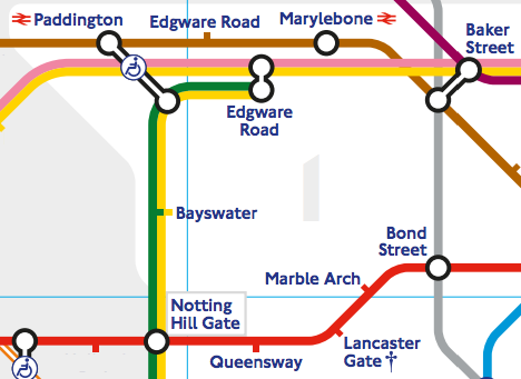
The London Undergroup map is 86 years old and is considered one of the great icons of British design. Virtually every public transportation map around the world is based upon its original schematic design.
It's pretty perfect for easily trying to find out which lines to take and which stations to transfer at to get across London however what it doesn't show, is the relative distances and travel times between each of those stations which can sometimes lead to suboptimal route planning.
For example, to get from Paddington to Bond Street, there are two clear (seemingly equidistant) routes on the map; via Baker St or via Notting Hill Gate. As we will explore, they are not equidistant and can significantly exacerbate journey time if the wrong route is chosen.
To visualise the underground map using the cleaned dataset from Part One, we need the list of stations along with
the possible links from each station to another. It's enough to just look at the longest "inbound" route for each line because (we would hope) that the "outbound" route is identical. This is provided by the inbound_graph PostgreSQL view.
First, create an empty MultiGraph which allows for multiple links between two stations. For instance, Liverpool St to Farringdon is served by three separate lines.
import networkx as nx
G = nx.MultiGraph()
Now, query the database and add both stations and the edge between them to the graph object.
import psycopg2
import psycopg2.extras

conn = psycopg2.connect(host="localhost",database="londontubepython", user="postgres", password="mysecretpassword")
cur = conn.cursor('server_side_cursor', cursor_factory=psycopg2.extras.DictCursor)
cur.execute("SELECT * FROM inbound_graph")

# Loop through the dataset adding StopPoints if they don't already exist with an edge for each row
for row in cur:
    if row['From_StopPointName'] not in G:
        G.add_node(row['From_StopPointName'], lon = row['From_Longitude'], lat = row['From_Latitude'])
    if row['To_StopPointName'] not in G:
        G.add_node(row['To_StopPointName'], lon = row['To_Longitude'], lat = row['To_Latitude'])
    G.add_edge(row['From_StopPointName'], row['To_StopPointName'], line = row['Line'])

cur.close()
conn.close()
print(nx.info(G))
So for the 269 tube stations we're visualising 429 of the links between them (as there are more links by including outbound routes too).
Let's start with a simplistic plot of the 250miles of tube network:
from matplotlib import pyplot as plt
from networkx.drawing.nx_agraph import graphviz_layout
%matplotlib inline

options = {
    'width': 1,
    'alpha': 0.3,
}

plt.subplots(figsize=(6,6))
nx.draw_networkx_edges(G, pos = nx.spring_layout(G), **options)
plt.tight_layout()
plt.axis('off');

Not exactly an icon of British design though we can see which routes serve multiple lines with the darkness of the edges.
Let's change the layout and add some colour. (Of course, somewhere in the internet archives sit the official TfL colour standards...)
# Map each Line to TfL's published RBG values
line_colours = {
        'VIC': (0, 160, 226),
        'PIC': (0, 25, 168),
        'WAC': (118, 208, 189),
        'NTN': (0, 0, 0),
        'HAM': (215, 153, 175),
        'BAK': (137, 78, 36),
        'CIR': (255, 206, 0),
        'DIS': (0, 114, 41),
        'CEN': (220, 36, 31),
        'JUB': (134, 143, 152),
        'MET': (117, 16, 86),
}
# Convert RGB to [0,1] scale
line_colours = {line: tuple([x / 255.0 for x in rgb]) for line, rgb in line_colours.items()}

options = {
    'edges': G.edges(),
    'edge_color': [line_colours[data['line']] for u,v,data in G.edges(data=True)],
    'width': 1.5,
    'alpha': 1,
}
plt.subplots(figsize=(10,10))
nx.draw_networkx_edges(G, pos = graphviz_layout(G, prog = 'neato'), **options)
plt.tight_layout()
plt.axis('off');

Even without any station labels can now discern some of the key features of the network.
- The top left corner is the Heathrow Airport loop on the Piccadily line
- Proximity-wise, that makes the termini clock-wise and to the right Ealing Broadway and West Ruislip
- The Circle line shares its route with the Hammersmith and City line on its way to...Hammersmith whilst the Picadilly and Metropolitan lines are the same towards Uxbridge.
- The northeastern loop of the Central line out to Woodford and Epping is in the lower right
Despite these key features, the layout clearly represents nothing geographic. The Metropolitan line in the top right of the graph is in the North West corner of London so the Jubilee line that joins it will be the Stanmore end. The next intersection along (clockwise) is the Northern line intersecting with the second stop of the Victoria line and therefore must be Stockwell next to Brixton on the completely opposite side of London.
Here's the same layout with labels for the stations mentioned:
nodes_to_label = ['Heathrow Terminals 1-3', 'Ealing Broadway', 'West Ruislip', 'Bank',
                  'Hammersmith (Ham & City Line)', 'Uxbridge Station', 'Woodford', 'Epping', 'Amersham',
                  'Stanmore', 'Stockwell Station', 'Brixton']

options['width'] = 3
options['alpha'] = 0.3

labels = {}
for node in G.nodes():
    if node in nodes_to_label:
        labels[node] = node

plt.subplots(figsize=(12,8))
pos = graphviz_layout(G, prog = 'neato')
nx.draw_networkx_edges(G, pos = pos, **options)
nx.draw_networkx_labels(G, pos, labels, size = 12, weight = 'heavy')
plt.tight_layout()
plt.axis('off');

The last step would be to add some realism by showing what the famous tube map doesn't show: the actual positions of stations on a map of London. The node positions are redefined as Longitude and Latitude coordinates and plotted against a Leaflet map of London.
pos = {node: (data['lon'], data['lat']) for node, data in G.nodes(data=True)}

import mplleaflet
plt.subplots(figsize=(10,10))
nx.draw_networkx_edges(G, pos = pos, width = 2., edge_color = options['edge_color'])
mplleaflet.display(tiles='cartodb_positron')
Here's that infamous section of the network where 30% of people go the wrong way:
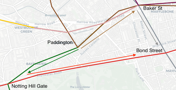
Now it seems much clearer which route takes 15mins and which takes 8mins!
Journey Planner Algorithm
This goal of this section is to compare a simple API call and parsing of JSON results (Week 5) to an example of sophisticated usage for the prepared timetable data from Part One with the help of the Departures Board query illustrating advanced SQL functionality.
Eyeballing a geographically-accurate map of the network isn't really the best way to work out the fastest route from Paddington to Bond Street. The more accurate way would be to weight each edge of our network by the travel time between the two stations and then use a shortest path graph algorithm to find the sequence of edges from station A to station B with the smallest total weight (ie travel time).
It's worth noting that despite the misleading name of "shortest path", since we don't really care how far we travel, we want to weight by time rather than distance to get to our destination the fastest way, not the shortest way.
There is one more factor to consider though because modelling the shortest path this way assumes that there is a train ready and waiting to go the moment you want to leave and at every station at which you transfer. With the exception of the Central line in peak hour, this is almost never the case in any transportation network.
Formulation
We model the tube stations using a time-expanded graph network where each node represents a station-event rather than a station. In other words, there is a "Hyde Park Corner" node for every arrival and departure of every vehicle into and out of that station. When we lumped WaitTime in with RunTime to create JourneyTime, we simplified the problem to assume that the train's arrival and departure is instantaneous so there's no need to create both a departure and arrival node.
We then we have two types of edges:
- Travel Edge: Represents the movement of a train from one station to the next
- Stay Edge: Represents waiting at a station for the immediately next train to depart. Effectively these are chained between all successive departures out of a given station throughout the day so that we can wait for any successive train at that station and not just the very next one to leave.
This does however assume that there is negligible transfer time within a station (when it actually takes +5mins to walk from the Victoria line to the Metropolitan line at King's Cross).
Due to the size of the Departures Board, we'll extract the full network timetable just for Monday 15th Jan 2018:
timetable_date = '2018-01-15'

# Placeholder for timetable_date in the table-valued function `departureboard`
sqlquery = ('SELECT * FROM departureboard(%s) '
            'ORDER BY "From_StopPointName", "DepartureMins_Link", "VehicleJourneyCode" ')
import networkx as nx
import psycopg2
import psycopg2.extras
Unlike the Tube Map model, we want to model the network using a Directed Graph instead of a Multi Graph because each train is travelling in a specific direction and no vehicle travels the same link at the same time.
Looping through each row in the Departure Board query we add a node for each station-vehicle pair. In the case where the station is the terminus, we need to add the arrival node as well as the departure node.
The first edge added is simply the train's movement between stations whereas the second edge is the 'stay' edge from that train's arrival to the next train's departure from the same station.
H = nx.DiGraph()

from copy import copy
prev_row = None

conn = psycopg2.connect(host="localhost",database="londontubepython",
                        user="postgres", password="mysecretpassword")
cur = conn.cursor('server_side_cursor', cursor_factory=psycopg2.extras.DictCursor)
cur.execute(sqlquery, (timetable_date,))

for row in cur:

    # Add or update node data for the Departure node in this row
    H.add_node(row['VehicleJourneyCode'] + '//' + row['From_StopPointRef'],
               VehicleJourneyCode = row['VehicleJourneyCode'],
               StopPointName = row['From_StopPointName'],
               MinuteOfDay = row['DepartureMins_Link'])

    # If this is the last stop for a train then add or update
    # node data for the Arrival node in this row
    if row['Flag_LastStop'] == True:
        H.add_node(row['VehicleJourneyCode'] + '//' + row['To_StopPointRef'],
               VehicleJourneyCode = row['VehicleJourneyCode'],
               StopPointName = row['To_StopPointName'],
               MinuteOfDay = row['ArrivalMins_Link'])

    # Create Travel edge
    H.add_edge(row['VehicleJourneyCode'] + '//' + row['From_StopPointRef'],
               row['VehicleJourneyCode'] + '//' + row['To_StopPointRef'],
               movement = row['Line'],
               # Edge weight is the travel time between stations
               cost = row['JourneyTime'])

    # Create Stay edge from the previous departure row provided it's the same station
    # NB: The result set is ordered by Departure Station, Departure Time so every station's
    #     departures are grouped and ordered together.
    if prev_row is not None and prev_row['From_StopPointName'] == row['From_StopPointName']:
        H.add_edge(prev_row['VehicleJourneyCode'] + '//' + prev_row['From_StopPointRef'],
                   row['VehicleJourneyCode'] + '//' + row['From_StopPointRef'],
                   movement = 'Stay',
                   # Edge weight is the waiting time between departures
                   cost = row['DepartureMins_Link'] - prev_row['DepartureMins_Link'])

    prev_row = copy(row)


cur.close()
conn.close()
We're now ready to query the timetable.
The query format contains the start and end stations with the departure time in minutes after midnight.
Once that's provided, we can modify the graph with two 'helper' nodes ('Start and 'End') which signify the origin and destination
of the query. These are then linked to each of their station's vehicle departures and arrivals respectively.
Currently these are matched partially using an in clause such that querying Liverpool St matches any node Liverpool St... and while this isn't very robust it allows for shortening station names.
We can also specify whether the intention is to leave from the origin after the specified time or to arrive at the destination prior to time with the leave_after parameter.
path_query = {
    'From_StopPointName': 'Liverpool St', # Actual station name is Liverpool Street Station
    'To_StopPointName': 'Hyde Park', # Actual station name is Hyde Park Corner
    'time': 23 * 60, # Provided in minutes past midnight
    'leave_after': True # Leave after or Arrive before
}
def setup_shortest_path(path_query):
    """
        Add the Start and End nodes to the network for the given query
        Connect them to the departures and arrivals for the relevant stations
    """

    # For "Leave After" query, assign the leaving time to the start node and
    # leave arriving time as unknown
    if path_query['leave_after'] == True:
        H.add_node('Start', StopPointName = path_query['From_StopPointName'],
                   MinuteOfDay = path_query['time'], movement = 'Departure')
        H.add_node('End', StopPointName = path_query['To_StopPointName'],
                   MinuteOfDay = None, movement = 'Arrival')

    # For "Arrive Before" query, assign the arriving time to the end node and
    # leave departure time as unknown
    else:
        H.add_node('Start', StopPointName = path_query['From_StopPointName'],
                   MinuteOfDay = None, movement = 'Departure')
        H.add_node('End', StopPointName = path_query['To_StopPointName'],
                   MinuteOfDay = path_query['time'], movement = 'Arrival')

    for n, n_data in H.nodes(data=True):
        # Don't want to add an edge from 'Start' to 'End', 'End' to 'End' or
        # 'Start' to 'Start'
        if n == 'Start' or n == 'End':
            continue

        if path_query['leave_after'] == True:
            # Cannot catch a train that has already left
            if n_data['MinuteOfDay'] >= path_query['time']:

                if path_query['From_StopPointName'] in n_data['StopPointName']:
                    H.add_edge('Start', n, movement = 'Start',
                               cost = n_data['MinuteOfDay'] - path_query['time'])

                if path_query['To_StopPointName'] in n_data['StopPointName']:
                    H.add_edge(n, 'End', movement = 'End', cost = 0)

        else:

            # No point catching a train that leaves after we want to arrive
            if n_data['MinuteOfDay'] <= path_query['time']:

                if path_query['From_StopPointName'] in n_data['StopPointName']:
                    H.add_edge('Start', n, movement = 'Start', cost = 0)

                if path_query['To_StopPointName'] in n_data['StopPointName']:
                    H.add_edge(n, 'End', movement = 'End',
                               cost = path_query['time'] - n_data['MinuteOfDay'])
Next, due to the formulation of our network, the raw path result isn't going to be terribly pretty so we can define some conditions to print only the information an end-user wants to know; when to get on or off a train.
def minutes_to_time(minutes_past_midnight):
    """
        Reformat a decimal 'minutes past midnight' to a time string rounded to the nearest second
    """
    hours, remainder = divmod(minutes_past_midnight * 60, 3600)
    minutes, seconds = divmod(remainder, 60)
    return '{:02.0f}:{:02.0f}:{:02.0f}'.format(hours, minutes, int(seconds))


def print_path(path):
    """
        Iterate through a journey's shortest path and print only the relevant information
        ie. When to board a train, change trains or leave a station
    """
    for u,v in zip(path,path[1:]):
        u_data = H.nodes(data=True)[u]
        v_data = H.nodes(data=True)[v]
        edge_data = H[u][v]

        # Starting information
        if edge_data['movement'] == 'Start':
            print('Start journey from {} at {}\n'\
            .format(u_data['StopPointName'], minutes_to_time(v_data['MinuteOfDay'] - edge_data['cost'])))

        # Changing onto a train from waiting at a platform
        elif previous_edge['movement'] == 'Start' or \
                (previous_edge['movement'] == 'Stay' and \
                 previous_edge['movement'] != edge_data['movement']):
            print('Board the {:>7} line train from {} at {}'.format(edge_data['movement'], u_data['StopPointName'], minutes_to_time(u_data['MinuteOfDay'])))

        # Changing off a train from travelling through any number of stops
        elif edge_data['movement'] != previous_edge['movement'] and edge_data['movement'] == 'Stay':
            print('Disembark the {:>3} line train at {} at {}'.format(previous_edge['movement'], u_data['StopPointName'], minutes_to_time(u_data['MinuteOfDay'])))

        # Finishing information
        elif edge_data['movement'] == 'End':
            print('\nFinish journey at {} at {}'.format(u_data['StopPointName'], minutes_to_time(u_data['MinuteOfDay'])))

        previous_edge = edge_data
Finally, putting this all together we can define a "journey planner" function.
Running a query happens near-instantaneously as the network isn't very large even with the time-expanded formation as we have filtered down to one day. The SQL query to pull the Departures Board from the database is comparatively much slower.
def plan_journey(path_query):
    """
        Add Start and End nodes to the network temporarily based on `path_query`
        Calculate and print shortest path
        Remove Start and End nodes (along with any induced edges) to 'clean' network for next query
    """
    setup_shortest_path(path_query)
    path = nx.shortest_path(H, source='Start', target='End', weight='cost')
    print_path(path)
    H.remove_nodes_from(['Start', 'End'])
# Liverpool St to Hyde Park leaving after 11pm
plan_journey(path_query)
# Arrive before 11pm
path_query['leave_after'] = False
plan_journey(path_query)
# Heathrow to Canada Water leaving after 7:40:58pm
path_query['leave_after'] = True
path_query['From_StopPointName'] = 'Heathrow'
path_query['To_StopPointName'] = 'Canada Water'
path_query['time'] = 19.683 * 60
plan_journey(path_query)
In the event that you have to wait an extra four seconds for your baggage to appear at the carousel you'll want to take the District and Victoria lines instead of just the Jubilee line...
# Heathrow to Canada Water leaving after 7:41:02pm
path_query['time'] = 19.684 * 60
plan_journey(path_query)
...and just in case it wasn't already clear from a geographically accurate tube map...
path_query['time'] = 19.66 * 60
path_query['From_StopPointName'] = 'Paddington'
path_query['To_StopPointName'] = 'Bond'
plan_journey(path_query)
Finally we can compare this result with the official TfL Journey Planner:
import requests, json
paddington, bondst, = 1000174, 1000025
date, time = 20180115, 1941 # time is approximate since the actual Departure Time in the query result is 1940
query = ("https://api.tfl.gov.uk/Journey/JourneyResults/" +
        "{}/to/{}?date={}&time={}" +
        "&timeIs=Departing&journeyPreference=LeastTime")
query = query.format(paddington, bondst, date, time)
result = json.loads(requests.get(query).content)
best_journey = result['journeys'][0]
print('Deparure Time: ', best_journey['startDateTime'])
print('Leg 1: ', best_journey['legs'][0]['instruction']['summary'])
print('Leg 2: ', best_journey['legs'][1]['instruction']['summary'])
print('Arrival Time: ', best_journey['arrivalDateTime'])
This simple Journey Planner algorithm has provided the same finish time and route as the official TfL API!
Trains Moving Throughout the Network
The most complex visualisations of spatiotemporal data involve trying to look at the space and time dimensions simultaneously. The interactive javascript tube map seen earlier is a good way to visualise a static representation of the network however since we are working with timetable data which inheritantly contains the movement of trains over time then the final step would be to plot these train movements over time.
For the final section of the project, we will look at visualising the movement of tube vehicles across a map of central London over the course of a day.
Begin by choosing the date of timetables we want to visualise:
timetable_date = '2017-12-20'
We'll need to use our tube line graph G from the Tube Map section so ensure that is loaded first.
The Departures Board query from the Shortest Path section is also needed however this time the whole table is
to be loaded into a DataFrame.
Annoyingly pandas requires that every column be explicitly listed however this is much faster than the alternative of adding an SQLAlcehmy layer.
import pandas as pd

conn = psycopg2.connect(host="localhost", database="londontubepython", user="postgres", password="mysecretpassword")
cur = conn.cursor()
cur.execute('SELECT * FROM departureboard(%s)', (timetable_date,))

df = pd.DataFrame(cur.fetchall(), columns=['VehicleJourneyCode', 'Line', 'From_VehicleSequenceNumber',
'From_StopPointRef', 'From_StopPointName', 'From_Longitude', 'From_Latitude', 'To_VehicleSequenceNumber',
'To_StopPointRef', 'To_StopPointName', 'To_Longitude', 'To_Latitude', 'JourneyTime', 'DepartureMins_Link',
'ArrivalMins_Link', 'Flag_LastStop'])
The problem with the structure of the Departures Board query is that it's returned a dataset where every row constitutes the departure of a train from any station. In order to plot the train movements we need to know where they are between departures continuously. One train may leave one station at say 7:00pm and not arrive at the next station for 5 minutes meanwhile another train has visited three stations in that time.
This can be solved by pivotting the dataset from the point of view of a train time of departure to a train location by time.
Pivotting in this manner means that we need to choose a sampling frequency for the train location calculation. The dataset is already rounded to the nearest 60 seconds however some tube links only take 60 seconds to travel between which would cause the resulting animation to show trains teleporting between stations. Two clever values are to sample every 12 or 20 seconds because then two trains approaching each other from two stops that are 60 seconds apart won't overlap on the plot.
The other consideration when pivotting is that the dataset doesn't include the location of the terminus. The final row of a vehicle is the departure time of the penultimate stop with the arrival time of the terminus. Therefore we also need to pull out all these termini, shift the columns to align with the departures and append them onto the departures table.
# Select required columns
df_expanded = df[['VehicleJourneyCode', 'Line', 'Flag_LastStop', 'DepartureMins_Link', 'ArrivalMins_Link',
                  'From_Longitude', 'From_Latitude', 'To_Longitude', 'To_Latitude']]

# Subset to the last trip link of each vehicle and rename the "arrival" columns to be "departure" columns
# to allow for automatic concatenation by column name
columns_to_shift = {'ArrivalMins_Link':'DepartureMins_Link',
                    'To_Longitude':'From_Longitude',
                    'To_Latitude':'From_Latitude'}
df_laststop = df_expanded.loc[df_expanded['Flag_LastStop'] == True].drop(columns_to_shift.values(), axis=1)
df_laststop.rename(columns = columns_to_shift, inplace = True)
df_expanded = pd.concat([df_expanded.drop(columns_to_shift.keys(), axis=1), df_laststop])

# Cast the "DepartureMins_Link" column to be a TimeDelta object and set it as a MultiIndex with "VehicleJourneyCode"
df_expanded = df_expanded.set_index(pd.to_timedelta((df_expanded['DepartureMins_Link']).astype('int'), unit='m'))
df_expanded = df_expanded.groupby('VehicleJourneyCode')
def resample_vehicle_departures(df_expanded, sample_freq):
    """
        Input a DataFrame with a MultiIndex of VehicleJourneyCode with DepartureMins_Link
        Resample the time dimension for each vehicle every `sample_freq` seconds
        Interpolate vehicle location for the new sample_freq.
    """
    # Expand the trip start and end times of every "VehicleJourneyCode" by sample_freq seconds
    df_resampled = df_expanded.resample(str(sample_freq) + 'S').asfreq()

    # Fill in the Line for each vehicle
    df_resampled['Line'] = df_resampled['Line'].ffill().bfill()

    # Linearly interpolate the Latitude and Longitude
    df_resampled = df_resampled.interpolate(method='linear')

    # Drop unneeded columns
    df_resampled = df_resampled.drop(['VehicleJourneyCode', 'DepartureMins_Link', 'Flag_LastStop'], 1)
    df_resampled = df_resampled.reset_index()

    return df_resampled
sample_freq = 20 # interpolate the vehicle location every sample_freq seconds
df_resampled = resample_vehicle_departures(df_expanded, sample_freq)
# Show vehicle positions as at 12:03:40
h,m,s = 12,3,40
assert s % sample_freq == 0 # seconds are a multiple of sample_freq otherwise no data returned
time = pd.to_timedelta((h*60 + m)*60 + s, unit='s')
df_resampled.loc[df_resampled['DepartureMins_Link'] == time].head()
This dataset is now in the perfect structure for finding the exact location of any vehicle for any discrete
point in time by subsetting on the DepartureMins_Link column.
For the animation we'll need a few additional packages in addition to matplotlib.animation.
The smopy module provides the OpenStreetMap
tile which we'll be plotting on, numpy provides a useful function np.c_ for concatenating series and
IPython purely for displaying the final product in Jupyter.
import smopy
import numpy as np
from matplotlib import animation
from matplotlib import pyplot as plt
from IPython.display import HTML, Image
%matplotlib inline
Firstly, set the start and finish times of the animation.
# Set the animation start time in minutes past midnight
start_time = 5.5 * 60 # 5:30am
end_time = 8 * 60 # 8:00am
The create_train_timetable_animation function consists of four parts:
- Setting up the base layer of the plot
- Defining the initial state of the animation in
init - Defining what each sequential frame of the animation looks like for a given frame number
iwithanimate - Returning the
FuncAnimationobject for a given number of frames calculated from thestart_time,end_timeandsample_freq
The first part downloads the same OSM layer we used for the Tube Network previously but using smopy
and then defines the region of interest as central London. Then setup the plot area, add the map layer
and plot an empty scatter plot with an empty annotation. The scatter will show the locations of each train
and the annotation will tell us the time of day for that frame.
The init function is just a replica of the Tube Map plot as this will be part of the base layer with
a change to the alpha level to make it more faint.
The animate function takes a frame number as input, calculates the current time using the start time
and sample_freq and subsets df_resampled to the vehicle positions at that time. Finally we map the
latitude and longitude coordinates to pixel positions on the plot, map the tube line to an RGB colour
and plot!
seconds_in_minute = 60
seconds_in_hour = 3600
def convert_to_time(timedelta):
    """
        Convert timedelta "seconds past midnight" object to an (H,M,S) tuple
    """
    hours, remainder = divmod(timedelta.seconds, seconds_in_hour)
    minutes, seconds = divmod(remainder, seconds_in_minute)
    return hours, minutes, seconds

def create_train_timetable_animation(start_time, end_time):
    """
        Returns an animation object plotting the movement of trains across
        a map of central London between start_time and end_time
    """
    # Setup
    smopy.TILE_SERVER = "http://tile.basemaps.cartocdn.com/light_all/{z}/{x}/{y}@2x.png"
    smopy.TILE_SIZE = 512

    # Set map bounds around central London
    map = smopy.Map((51.45, -0.3, 51.55, -0.05), z = 12)

    # Setup plot
    fig = plt.figure(figsize=(15, 15), dpi=None)
    ax = plt.subplot(111)
    plt.xticks([])
    plt.yticks([])
    plt.grid(False)
    plt.xlim(0, map.w)
    plt.ylim(map.h, 0)
    plt.axis('off')
    plt.tight_layout()
    ax = map.show_mpl(ax=ax)

    # Draw baselayer
    options['alpha'] = 0.2
    pos = {node: map.to_pixels(data['lat'], data['lon']) for node, data in G.nodes(data=True)}
    nx.draw_networkx_edges(G, pos = pos, **options)

    # Initialise animation objects
    x, y, c = [],[],[]
    scat = ax.scatter(x=x,y=y,c=c,s=12)
    current_time = ax.text(35, 70, s='', fontsize=18)

    def init():
        """
            Background of each frame to be cached
        """
        scat.set_offsets([])
        current_time.set_text('')
        return scat,current_time

    minutes_to_animate = end_time - start_time
    def animate(i):
        """
            Returns animation state for a given frame i
        """
        # Calculate the time (in seconds past midnight) of the frame number
        # by using the sample_freq of df_resampled
        time_now = start_time * seconds_in_minute + i * sample_freq

        # Cast time to a timedelta object and subset df_resampled
        time_td = pd.to_timedelta(time_now, unit='s')
        df_now = df_resampled.loc[df_resampled['DepartureMins_Link'] == time_td]

        # Map lat, lon and colours
        x_pixel, y_pixel = map.to_pixels(df_now['From_Latitude'], df_now['From_Longitude'])
        frame_colouring = df_now['Line'].map(line_colours)

        # Plot frame
        scat.set_offsets(np.c_[x_pixel, y_pixel])
        scat.set_color(frame_colouring)
        current_time.set_text('{:02d}:{:02d}:{:02d}'.format(*convert_to_time(time_td)))

        return scat,current_time

    # Animate with the number of frames calculated from start_time, end_time and sample_freq
    # blit = True means only re-draw the parts that have changed
    anim = animation.FuncAnimation(fig, animate, init_func=init, interval=60, blit=True,
                                   frames = int(minutes_to_animate*(seconds_in_minute/sample_freq)))
    return anim
To see this is action, let's look at three key periods of the day.
First thing in the morning...
4:45am to 7:00am
%%capture
start_time, end_time = 4.75 * 60, 7 * 60
anim_early = create_train_timetable_animation(start_time, end_time);
anim_early.save('anim_early.mp4', writer='ffmpeg');
%%HTML
<video width="700" height="700" controls>
  <source src="anim_early.mp4" type="video/mp4">
</video>
... peak hour in the afternoon ...
5:30pm to 6:30pm
%%capture
start_time, end_time = 17.5 * 60, 18.5 * 60
anim_peak = create_train_timetable_animation(start_time, end_time);
anim_peak.save('anim_peak.mp4', writer='ffmpeg');
%%HTML
<video width="700" height="700" controls>
  <source src="anim_peak.mp4" type="video/mp4">
</video>
... and last thing at night.
11:30pm to 1:30am
%%capture
start_time, end_time = 23.5 * 60, 25.5 * 60
anim_late = create_train_timetable_animation(start_time, end_time);
anim_late.save('anim_late.mp4', writer='ffmpeg');
%%HTML
<video width="700" height="700" controls>
  <source src="anim_late.mp4" type="video/mp4">
</video>
In this last plot, the timedelta object will handle the end_time wrapping to the next day because it converts it back to the start of our dataset. There's no jump in any of the train positions at midnight because the timetable for the
21st December is probably identical to 20th December with them both being weekdays. It may be a different story if plotting a Sunday night into a Monday morning.
Of course, if you really wanted, you could sit and watch an entire day of train movements compressed into 4 minutes...
%%HTML
<video width="900" height="800" controls>
  <source src="tube_animation.mp4" type="video/mp4">
</video>
That concludes Part Two and this London Underground project!
Although only a couple of uses for the data have been shown here, there are naturally infinitely more visualisations possible such as examining the network properties of the Underground; the betweeness centrality and page rank of each station, how vertex degree correlates with train arrival frequency or how the distribution of vehicles within the network at any one time varies throughout the course of the week.